Opening Data:

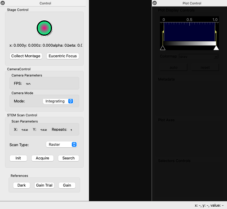
This example demonstrates how to open and visualize data using the SpyDE application.

We will start by opening the SpyDE main window as shown below.

CPU Count: 3
[startup] Plot update worker thread start completed in 0.0 ms
[startup] Plot control dock creation completed in 10.4 ms
[startup] Inst. control dock creation completed in 40.1 ms
Starting Dask LocalCluster with 1 workers, and 1 threads per worker

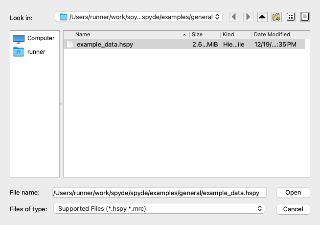
Here we have the SpyDE main window opened! Now, let’s open some example data. We can do this by navigating to the “File” menu and selecting “Open”. SpyDe can open all the file formats supported by HyperSpy. That being said, files which support distributed loading will work much better. If there is a specific file format that you would like to see supported, please open an issue on the RosettaSciIo GitHub page.

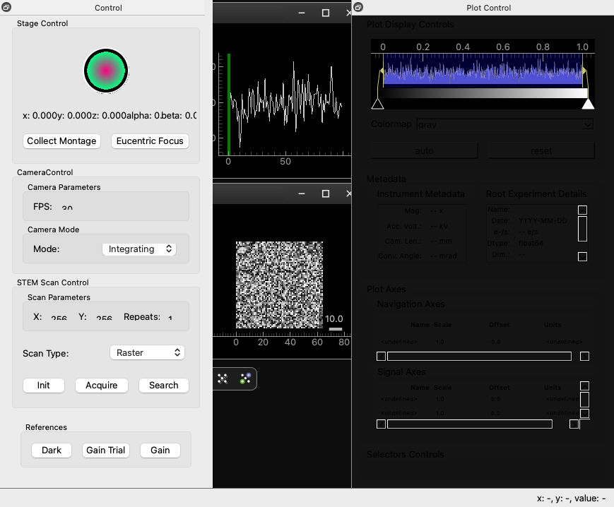
Now we can see the opened data in the SpyDE application!

Emitting Future, write_shared_array-a3af8dda0b24f09bd985bdebf343cace for plot: <spyde.drawing.plots.plot.Plot(0x160a39d40, parent=0x160a13bb0, pos=12,12, flags=(ItemUsesExtendedStyleOption|ItemSendsGeometryChanges)) at 0x1610a5100>
Read shared array in 0.03 ms
Emitting Future, finalize-hlgfinalizecompute-f035477fc02845b5ba1b82281eecc107 for plot: <spyde.drawing.plots.plot.Plot(0x15efa8ce0, parent=0x160a050c0, pos=12,12, flags=(ItemUsesExtendedStyleOption|ItemSendsGeometryChanges)) at 0x160672180>
Transferred Future over TCP in 2.55 ms
Updating Plot from worker signal...
Setting image data with img [[0.74432183 0.6325225  0.7493633  ... 0.03410073 0.77640999 0.89044296]
 [0.29414328 0.73027308 0.10093151 ... 0.95131195 0.10743438 0.17023182]
 [0.97448146 0.53891391 0.54407824 ... 0.35836436 0.77254874 0.98809062]
 ...
 [0.75282424 0.32024453 0.81422023 ... 0.79755846 0.3718993  0.10648215]
 [0.73897944 0.3522312  0.68877525 ... 0.13174099 0.30278926 0.23853144]
 [0.49496252 0.52097277 0.13448287 ... 0.14393519 0.17246608 0.91782443]]
setImage took 0.06ms
Updating Plot from worker signal...
Setting levels: (0.0004934051210775392, 0.9999460260860547) percentiles: (np.float64(0.1708984375), 100.0) on plot: <spyde.drawing.plots.plot.Plot(0x160a39d40, parent=0x160a13bb0, pos=12,12, flags=(ItemUsesExtendedStyleOption|ItemSendsGeometryChanges)) at 0x1610a5100>

We can now explore and visualize the data using SpyDE’s powerful tools and features!

Shutting down Dask cluster and client...

sphinx_gallery_thumbnail_number = 2