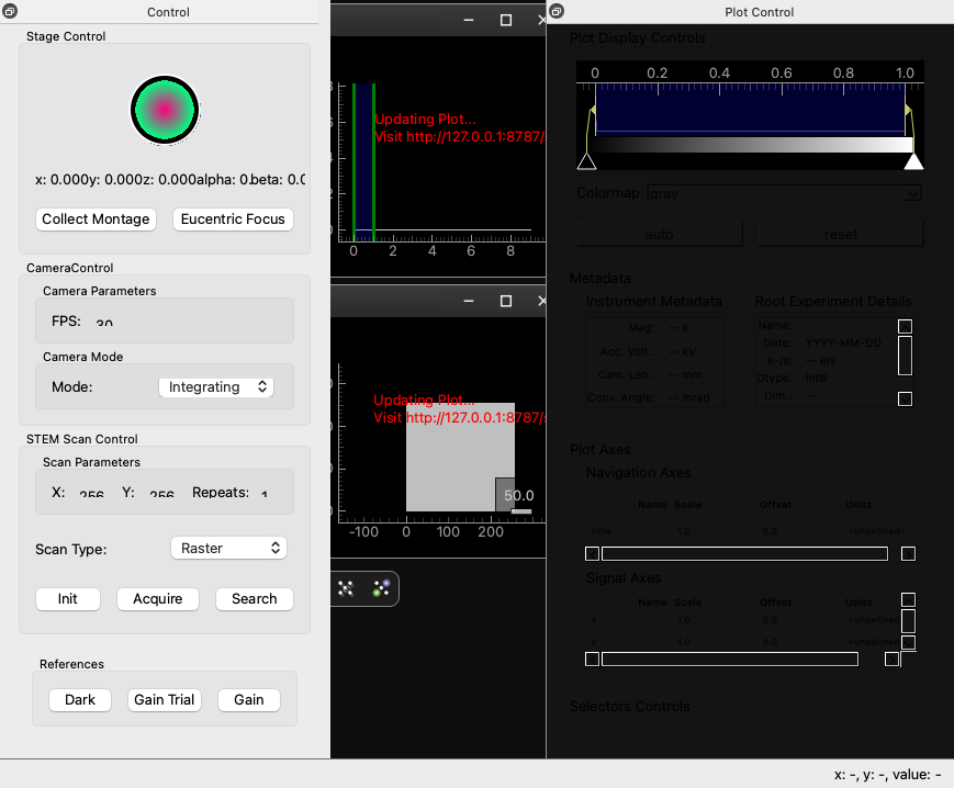
Changing Scales and Axes

This example demonstrates how to modify the scales and axes of a plot. These are rendered as QLabels but can be edited by left-clicking on them which will change them into QLineEdits for text input.

CPU Count: 3
[startup] Plot update worker thread start completed in 0.1 ms
[startup] Plot control dock creation completed in 23.1 ms
Starting Dask LocalCluster with 1 workers, 1 threads per worker
Creating Data
Dialog accepted
Data created
Creating Signal Tree for signal
Dask cluster ready. Dashboard: http://127.0.0.1:8787/status
MainWindow: Dask ready.
Initializing navigator for root signal:  <LazySignal2D, title: , dimensions: (10|256, 256)>
Navigator initialized:  [<LazySignal1D, title: , dimensions: (|10)>]
{<spyde.drawing.plots.plot.Plot(0x160e97100, parent=0x160eb9d30, pos=12,12, flags=(ItemUsesExtendedStyleOption|ItemSendsGeometryChanges)) at 0x1614b6f40>: [(0, 0)]}  after adding item at ( 0 , 0 )
Adding navigation plot states for signals: [<LazySignal1D, title: , dimensions: (|10)>]
{<spyde.drawing.plots.plot_window.PlotWindow(0x160e66970) at 0x16140c780>: {}}
Adding navigation plot state for plot: <spyde.drawing.plots.plot.Plot(0x160e97100, parent=0x160eb9d30, pos=12,12, flags=(ItemUsesExtendedStyleOption|ItemSendsGeometryChanges)) at 0x1614b6f40>
Plot states {}
SubTB: [[]]
SubTB: [[], []]
SubTB: [[], [], []]
SubTB: [[], [], [], []]
SubTB: [[], [], [], [], []]
Adding toolbar action: Reset to right toolbar
Function: functools.partial(<function reset_view at 0x1500cfa60>, action_name='Reset'), Icon: /Users/runner/work/spyde/spyde/spyde/drawing/toolbars/icons/fullsize.svg, Toggle: False, Params: {}
Adding toolbar action: Zoom In to right toolbar
Function: functools.partial(<function zoom_in at 0x1500cfba0>, action_name='Zoom In'), Icon: /Users/runner/work/spyde/spyde/spyde/drawing/toolbars/icons/zoom.svg, Toggle: False, Params: {}
Adding toolbar action: Zoom Out to right toolbar
Function: functools.partial(<function zoom_out at 0x1500cfb00>, action_name='Zoom Out'), Icon: /Users/runner/work/spyde/spyde/spyde/drawing/toolbars/icons/zoomout.svg, Toggle: False, Params: {}
Adding toolbar action: Add Selector to right toolbar
Function: functools.partial(<function add_selector at 0x1500cfc40>, action_name='Add Selector'), Icon: /Users/runner/work/spyde/spyde/spyde/drawing/toolbars/icons/add_selector.svg, Toggle: False, Params: {}
Adding toolbar action: Select Navigator to right toolbar
Function: functools.partial(<function toggle_navigation_plots at 0x1500cfd80>, action_name='Select Navigator'), Icon: /Users/runner/work/spyde/spyde/spyde/drawing/toolbars/icons/navigator.svg, Toggle: True, Params: {}
Initialized PlotState: <PlotState signal=<LazySignal1D, title: , dimensions: (|10)>, dimensions=1, dynamic=False>
setting Plot states:  {<LazySignal1D, title: , dimensions: (|10)>: <PlotState signal=<LazySignal1D, title: , dimensions: (|10)>, dimensions=1, dynamic=False>}  to signal: <LazySignal1D, title: , dimensions: (|10)>
updating data for static plot state... [<Future: pending, key: finalize-hlgfinalizecompute-82fa172ffd2443428b0bc220f875a29e>]
Updating plot data [<Future: pending, key: finalize-hlgfinalizecompute-82fa172ffd2443428b0bc220f875a29e>]  force= False
Updating 1D plot with axis: [0. 1. 2. 3. 4. 5. 6. 7. 8. 9.]
Data shape: [1. 1. 1. 1. 1. 1. 1. 1. 1. 1.]
The view range: [[0, 1], [0, 1]]
Setting current data to: <Future: pending, key: finalize-hlgfinalizecompute-82fa172ffd2443428b0bc220f875a29e>
Plot data updated.
Parent selector None
Delayed updating data for plot state: <PlotState signal=<LazySignal1D, title: , dimensions: (|10)>, dimensions=1, dynamic=False>
<pyqtgraph.graphicsItems.ImageItem.ImageItem(0x16173f9f0, pos=0,0, flags=(ItemSendsGeometryChanges)) at 0x16143b6c0>
Showing toolbars for plot state: <PlotState signal=<LazySignal1D, title: , dimensions: (|10)>, dimensions=1, dynamic=False>
Adding navigation selector to plot window: <spyde.drawing.plots.plot_window.PlotWindow(0x160e66970) at 0x16140c780>  with dim: 1
Plot window level: 1  children dict: {}
{<spyde.drawing.plots.plot_window.PlotWindow(0x160e66970) at 0x16140c780>: {}}
1
{<spyde.drawing.plots.plot.Plot(0x160e84050, parent=0x1612df9c0, pos=12,12, flags=(ItemUsesExtendedStyleOption|ItemSendsGeometryChanges)) at 0x161440200>: [(0, 0)]}  after adding item at ( 0 , 0 )
Hiding [<pyqtgraph.graphicsItems.LinearRegionItem.LinearRegionItem(0x160ef2970, parent=0x160e92710, pos=0,0, flags=(ItemSendsGeometryChanges)) at 0x1615bad40>]
Plot states {}
SubTB: [[]]
SubTB: [[], []]
SubTB: [[], [], []]
SubTB: [[], [], [], []]
SubTB: [[], [], [], [], []]
SubTB: [[], [], [], [], [], []]
SubTB: [[], [], [], [], [], [], []]
add_virtual_image
{'add_virtual_image': {'name': 'Add Virtual Image', 'description': 'Adds a virtual image from the 4D-STEM data.', 'icon': 'drawing/toolbars/icons/zoom.svg', 'function': 'spyde.actions.pyxem.add_virtual_image'}}
Sub Entries [(functools.partial(<function add_virtual_image at 0x161428cc0>, action_name='add_virtual_image'), '/Users/runner/work/spyde/spyde/spyde/drawing/toolbars/icons/zoom.svg', 'Add Virtual Image', False, {})]
SubTB: [[], [], [], [], [], [], [], [(functools.partial(<function add_virtual_image at 0x161428cc0>, action_name='add_virtual_image'), '/Users/runner/work/spyde/spyde/spyde/drawing/toolbars/icons/zoom.svg', 'Add Virtual Image', False, {})]]
add_line_profile
{'add_line_profile': {'name': 'Add Line Profile', 'description': 'Add a line profile ROI to the plot.', 'icon': 'drawing/toolbars/icons/line_profile.svg', 'function': 'spyde.actions.line_profile.add_line_profile'}}
Sub Entries [(functools.partial(<function add_line_profile at 0x1614296c0>, action_name='add_line_profile'), '/Users/runner/work/spyde/spyde/spyde/drawing/toolbars/icons/line_profile.svg', 'Add Line Profile', False, {})]
SubTB: [[], [], [], [], [], [], [], [(functools.partial(<function add_virtual_image at 0x161428cc0>, action_name='add_virtual_image'), '/Users/runner/work/spyde/spyde/spyde/drawing/toolbars/icons/zoom.svg', 'Add Virtual Image', False, {})], [(functools.partial(<function add_line_profile at 0x1614296c0>, action_name='add_line_profile'), '/Users/runner/work/spyde/spyde/spyde/drawing/toolbars/icons/line_profile.svg', 'Add Line Profile', False, {})]]
SubTB: [[], [], [], [], [], [], [], [(functools.partial(<function add_virtual_image at 0x161428cc0>, action_name='add_virtual_image'), '/Users/runner/work/spyde/spyde/spyde/drawing/toolbars/icons/zoom.svg', 'Add Virtual Image', False, {})], [(functools.partial(<function add_line_profile at 0x1614296c0>, action_name='add_line_profile'), '/Users/runner/work/spyde/spyde/spyde/drawing/toolbars/icons/line_profile.svg', 'Add Line Profile', False, {})], []]
Traceback (most recent call last):
  File "/Users/runner/work/spyde/spyde/spyde/__main__.py", line 489, in create_data
    self.add_signal(data, navigators=navigators)
  File "/Users/runner/work/spyde/spyde/spyde/__main__.py", line 594, in add_signal
    signal_tree = BaseSignalTree(
                  ^^^^^^^^^^^^^^^
  File "/Users/runner/work/spyde/spyde/spyde/signal_tree.py", line 110, in __init__
    self._initialize_initial_plots()
  File "/Users/runner/work/spyde/spyde/spyde/signal_tree.py", line 120, in _initialize_initial_plots
    self.navigator_plot_manager = MultiplotManager(
                                  ^^^^^^^^^^^^^^^^^
  File "/Users/runner/work/spyde/spyde/spyde/drawing/plots/multiplot_manager.py", line 67, in __init__
    self.add_navigation_selector_and_signal_plot(
  File "/Users/runner/work/spyde/spyde/spyde/drawing/plots/multiplot_manager.py", line 249, in add_navigation_selector_and_signal_plot
    self.signal_tree.create_plot_states(plot=child)
  File "/Users/runner/work/spyde/spyde/spyde/signal_tree.py", line 414, in create_plot_states
    plot.add_plot_state(
  File "/Users/runner/work/spyde/spyde/spyde/drawing/plots/plot.py", line 329, in add_plot_state
    ps = PlotState(
         ^^^^^^^^^^
  File "/Users/runner/work/spyde/spyde/spyde/drawing/plots/plot_states.py", line 81, in __init__
    self._initialize_toolbars()
  File "/Users/runner/work/spyde/spyde/spyde/drawing/plots/plot_states.py", line 129, in _initialize_toolbars
    get_toolbar_actions_for_plot(self)
  File "/Users/runner/work/spyde/spyde/spyde/drawing/toolbars/plot_control_toolbar.py", line 86, in get_toolbar_actions_for_plot
    base_func = getattr(importlib.import_module(module_path), attr)
                        ^^^^^^^^^^^^^^^^^^^^^^^^^^^^^^^^^^^^
  File "/Library/Frameworks/Python.framework/Versions/3.11/lib/python3.11/importlib/__init__.py", line 126, in import_module
    return _bootstrap._gcd_import(name[level:], package, level)
           ^^^^^^^^^^^^^^^^^^^^^^^^^^^^^^^^^^^^^^^^^^^^^^^^^^^^
  File "<frozen importlib._bootstrap>", line 1204, in _gcd_import
  File "<frozen importlib._bootstrap>", line 1176, in _find_and_load
  File "<frozen importlib._bootstrap>", line 1140, in _find_and_load_unlocked
ModuleNotFoundError: No module named 'spyde.actions.find_vectors'

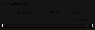
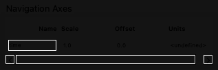
After opening the example data, we can see that the plot has default axis labels and scales. By left-clicking on the axis labels (e.g., “X Axis” or “Y Axis”), we can edit them to more meaningful names. Similarly, by left-clicking on the scale labels (e.g., “1.0” on the X-axis), we can change the scale values. This allows us to customize the plot to better represent the data being visualized.

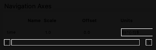
There is some limited support for mathematical expressions in the axis labels using LaTeX syntax. For example, we can label an axis as “$nm^{-1}$” to represent nanometers.

# After editing the axis labels and scales, the plot now reflects these changes with the updated labels and scales.
# This enhances the clarity and interpretability of the plot, making it easier to understand the data being presented.

Traceback (most recent call last):
  File "/Users/runner/work/spyde/spyde/spyde/drawing/signal_tree_presenter.py", line 30, in _on_axis_field_edit
    for plot in signal_tree.navigator_plot_manager.plots.values():
                ^^^^^^^^^^^^^^^^^^^^^^^^^^^^^^^^^^^^^^^^
AttributeError: 'NoneType' object has no attribute 'plots'

Finally, we can see the main window with the updated axis labels and scales reflected in the plot.